Table of Contents
Overview
This blog is inspired by one of the lectures by Ms Florina Pantilimonescu-Cioancă. Her idea is to prepare tutorial-style posts introducing mathematical concepts and then present them through BeeGraphy components. As a result to bring forth application for those notions. This blog explores the synergy between architecture and mathematics through her vision. And in the end we conclude with a small applied example of the Zayed Museum in Abu Dhabi.
Parametrization in Mathematics
In mathematics, we encounter two fundamental quantities when working with functions: variables and parameters.
The variable of a function, typically denoted as x, represents an independent quantity that is manipulated to evaluate the function. Consider a function of variable x,
f(x) = 2x² + 7x + 1
We substitute different values of x into the function to calculate the corresponding value of f(x). For instance, we might find f(0), f(1), or f(2) by plugging these values into our expression.
In contrast, parameters are the coefficients or constants that define the specific form of a function, commonly represented by letters like a, b, and c. The function f(x) = 2x² + 7x + 1 can be generalized as,
f(x) = ax² + bx + c,
Parameters are usually given implicitly and remain fixed. Though they don’t vary in typical problems, they serve a crucial role by allowing us to explore entire families of functions rather than just a single function.
By varying parameters, we can study how functions behave as a collective class, revealing new patterns and relationships.
Parameters in Architecture
In architecture, variables refer to changing conditions, such as how many people use a space at different times. A room may be empty, lightly occupied, or crowded, and architects consider these variations.
Parameters, in contrast, are fixed design constraints that define the framework. Elements like room size, ceiling height, column spacing, and structural grids remain constant once built. A parameter does not describe shape directly; instead, it sets the conditions under which shape is generated, determining what forms and uses are possible within the space.
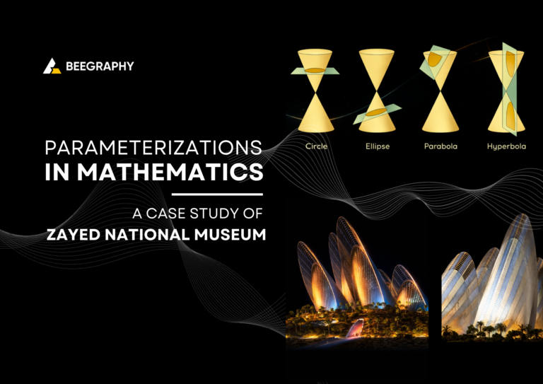
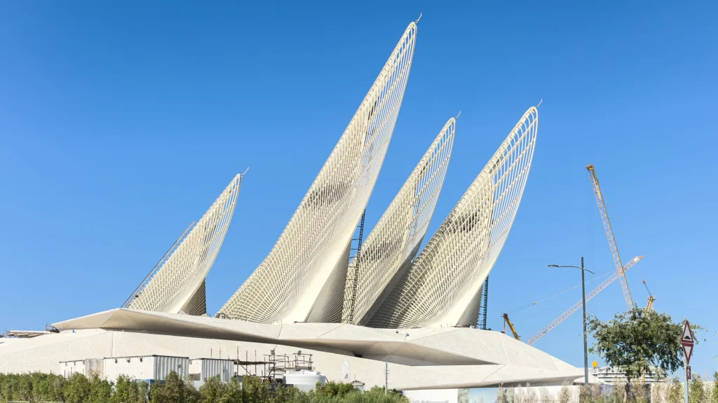
Take the example of Zayed National Museum, designed by Foster + Partners. It showcases parametric architecture through its wing-like towers, whose height, curvature, and spacing are treated as adjustable parameters to respond to climate, structure, and cultural expression.
Introduction to Conic Sections
Conic sections are one of the most important families of curves in mathematics. They are formed by the intersection of a plane with a double cone (two identical cones joined at their vertices) as shown in figure below.
Depending on the angle at which a plane slices through the cone, we obtain different members of the conic family:
- Circle: When the plane cuts perpendicular to the cone’s axis
- Ellipse: When the plane cuts at an angle, intersecting only one cone
- Parabola: When the plane is parallel to the slant of the cone
- Hyperbola: When the plane cuts through both cones
Creating Conic Sections With Beegraphy
Consider a cone with its center (vertex) at point O = (−20, 0, 0). We can explore different conic sections by intersecting this cone with three distinct planes, each defined by a point M on the plane and a normal vector N perpendicular to it:
Plane P₁: Point M₁ = (−20, 0, 5), Normal N₁ = (0, 0, 1)
This plane is horizontal (perpendicular to the z-axis), producing a circle
Plane P₂: Point M₂ = (−20, 0, 7), Normal N₂ = (0, 1, 1)
This tilted plane may produce an ellipse or parabola, depending on its angle relative to the cone.
Plane P₃: Point M₃ = (−20, 3, 0), Normal N₃ = (0, 1, 0)
This plane is perpendicular to the y-axis and could yield a hyperbola if it intersects both cones.
The General Form of Conic Equations
All conic sections can be described by a single general second-degree equation in two variables:
Ax² + Bxy + Cy² + Dx + Ey + F = 0
Here, A, B, C, D, E, and F are the parameters that determine which specific conic we obtain. This formulation shows that circles, ellipses, parabolas, and hyperbolas are all variations of the same fundamental equation. Thus giving us a parameterized family of curves.
To learn more about conic sections and how they behave. Check out this article. Conic section
Parametric Equation of Line
Consider a line in the plane that passes through the point M₀ = (2, 5) with direction vector v = 3i + 10j. We define this line parametrically using BeeGraphy.
The canonical equation of the line expresses the relationship between coordinates without an explicit parameter:
(x − x₀) / l = (y − y₀) / m
We begin with parametric equation of a line by introducing a parameter λ (lambda):
x = x₀ + λl
y = y₀ + λm
Here, λ ∈ ℝ is the parameter that traces out the entire line. Each value of λ corresponds to exactly one point on the line. λ shifts the line as we change its values in the direction of the vector.
Parametric Equation of Circle
We will define this circle parametrically using BeeGraphy and observe how varying the parameter t traces the circular path.
Consider a circle such that C(a, b) be a fixed point and r > 0 a fixed real number. The circle with center C and radius r is the geometric locus of all points M(x, y) that satisfy the equality:
|CM| = r …(i)
This definition states that a circle consists of all points at a constant distance r from the center C. Equation (i) is also equivalent to the parametric equations:
x = a + r cos t
y = b + r sin t
where t ∈ [0, 2π) is the parameter.
The parameter t represents the angle in radians measured counterclockwise from the positive x-axis. As t varies continuously from 0 to 2π, the point M(x, y) traces the entire circle exactly once in a counterclockwise direction. This is the geometric beauty of parametric representation, where circular motion emerges from the periodic nature of sine and cosine.
Parametric Equation of Ellipse
Now we will define this ellipse parametrically using BeeGraphy and observe how varying the parameter t traces the elliptical path.
Let C(h, k) be a fixed point and a > b > 0 be fixed real numbers.
- C(h, k) be a fixed point (center)
- a is the semi-major axis (horizontal radius)
- b is the semi-minor axis (vertical radius)
The ellipse is the geometric locus of all points M(x, y) that satisfy:
[(x − h)² / a²] + [(y − k)² / b²] = 1
The Cartesian equation is equivalent to the parametric equations:
x = h + a cos t
y = k + b sin t
where t ∈ [0, 2π) is the parameter.
The parameter t represents the angle parameter (not the geometric angle from the center, but the parameter of the ellipse). As t varies continuously from 0 to 2π, the point M(x, y) traces the entire ellipse exactly once in a counterclockwise direction.
Parametric Equation of Parabola
Consider a parabola with a vertex at O = (0, 0) and a directrix axis along OY (the y-axis). The parabola is the geometric locus of all points M in the plane with the property that the distance from M to the point F equals the distance from M to the line d. We will define this parabola parametrically in BeeGraphy and explore its geometric properties.
- The focus F: The fixed point from which distances are measured
- The directrix d: The fixed line from which distances are measured
- The parameter p: The distance from the focus to the directrix, denoted by p > 0
From the geometric definition, the equation of the parabola is derived:
y² = 4px
The equation y² = 4px can be expressed in parametric form. Let t be a parameter representing a vertical displacement. Then:
x = t²
y = 2pt
where t ∈ (−∞, +∞) is the parameter.
The parameter t represents a scaled vertical coordinate. As t varies continuously from −∞ to +∞, the point M(x, y) traces the entire parabola. Notice that both positive and negative values of t produce the same x-coordinate (since x = t²), generating the symmetric upper and lower branches simultaneously.
Parametric Equation of Hyperbola
The hyperbola is the geometric locus of all points M in the plane such that the absolute difference of the distances from M to the two foci is constant and equal to 2a. We will define this hyperbola parametrically in BeeGraphy and explore its geometric properties.
||MF₁| − |MF₂|| = 2a
- The foci F₁ and F₂: Two fixed points symmetric about the center
- The center O: The midpoint between the foci
- Semi-transverse axis a: Half the distance between the vertices
- Semi-conjugate axis b: Related to the “width” of the hyperbola
From the geometric definition, the standard Cartesian equation of the hyperbola with center at O(0, 0) and transverse axis along the x-axis is:
x²/a² − y²/b² = 1
The Cartesian equation can be expressed in parametric form using hyperbolic trigonometric functions:
x = a sec θ
y = b tan θ
where θ ∈ [0, 2π) with θ ≠ π/2, 3π/2
As t varies continuously from −∞ to +∞, the point M(x, y) traces the entire branches of the hyperbola.
Zayed National Museum
The Zayed National Museum can be read as a parametric system in which architectural form is created through geometric and spatial parameters.
The Five Falcon Wings: The museum’s most distinctive feature consists of five lightweight steel wings modeled after falcon feathers. They are defined by controllable variables such as height, curvature, orientation, and spacing, allowing the overall form to emerge from mathematical relationships between these parameters.
The Mound Structure: The museum spaces are housed within a faceted mound that abstracts the UAE’s desert topography. The geometric parameters of the mound – its slope angles, facet sizes, and material composition – were optimized to balance cultural symbolism with environmental efficiency.
Together, the wings and the mound form a unified geometric framework where changes in one parameter affect the entire system, leading to variations in spatial proportion and structural configuration.
Environmental performance is embedded within this parametric logic. Parameters such as tower height, vent placement, and section depth influence airflow and thermal behavior, showing how physical performance emerges from geometric control.
Key parameters of the museum include:
- Geometric: wing height, curvature, orientation
- Environmental: ventilation rates, cooling depths, thermal mass
- Spatial: gallery size, atrium volume, circulation patterns
- Material: white concrete with crushed marble, patinated bronze
By adjusting these parameters during design development, the architects explored multiple configurations, treating architecture as a flexible system rather than a single fixed form. Tryout with the Beegraphy model below to get a clearer understanding of how it works.
Step By Step Tutorial in BeeGraphy
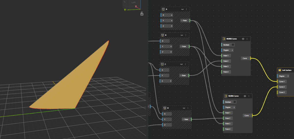
Base Structure
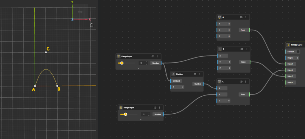
- Add Point A on the canvas. Treat this point as the origin to keep the setup simple.
- Add Point B along the x-axis only, at a chosen distance from Point A.
- Define Point C such that its x-coordinate lies exactly midway between Point A and Point B and its y-coordinate is offset by a chosen value in the same plane.
- To obtain the midpoint in the x-direction, use a Division node and divide the x-coordinate of Point B by 2.
- Assign this divided value as the x-coordinate of Point C.
- Specify the value of y-coordinate for Point C to complete its placement.
- Add a NURBS Curve component to the canvas. Define the curve to smoothly pass smoothly through A → C → B.
- Set Point A as Point 1 of the curve.
- Set Point C as Point 2 of the curve.
- Set Point B as Point 3 of the curve.

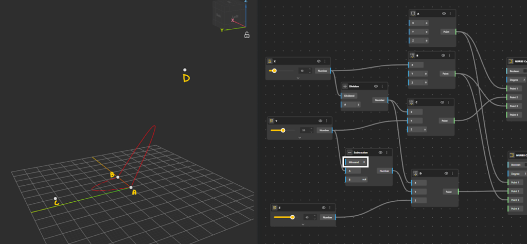
- Add Point D to the canvas using the Construct Point component.
- Define the x-coordinate of Point D identically to Point C (i.e., halfway between Point A and Point B).
- For the y-coordinate, take the offset in the opposite direction:
- Add a Subtraction node.
- Set the minuend to 0.
- Subtract the y-coordinate value to obtain a negative y value.
- To lift the point into 3D space, define the z-coordinate of Point D. Point D is now positioned symmetrically in y and elevated along the z-axis.
- Add a second NURBS Curve component to the canvas. The second curve is now defined, passing through A → D → B, forming a spatial (3D) curve.
- Set Point A as Point 1 of the curve.
- Set Point D as Point 2 of the curve.
- Set Point B as Point 3 of the curve.
- Add a Loft surface component to the canvas. Connect both NURBS curves as inputs to the Loft node. The Loft component generates a surface by smoothly interpolating between the two curves along their length.
Top Structure
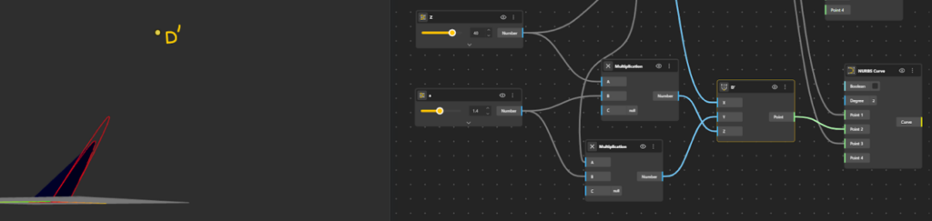
To Create the feather-like extension we will use the same base points as before.
The feather is simply an extension of the existing curve A–D–B. Therefore, D′ must lie in the same direction as D, not in a new direction. The direction of D relative to the base curve is already defined by its y and z coordinates. To extend the curve without changing its direction, we do not redefine these coordinates. Instead, we scale them. This is done by multiplying the y and z values of D by an amplitude factor a. The x-coordinate is kept the same, so the extension happens outward, not along the curve length.
D′=(x, ay, az)
Since both coordinates are scaled by the same factor, the point moves further along the same line of action.
- Add Construct Point component to define Point D′.
- Keep the x-coordinate of D′ the same as Point D.
- Introduce an amplitude factor, call it a.
- Apply this amplitude to both the y-coordinate and z-coordinate:
- Multiply the original y-value by a
- Multiply the original z-value by a
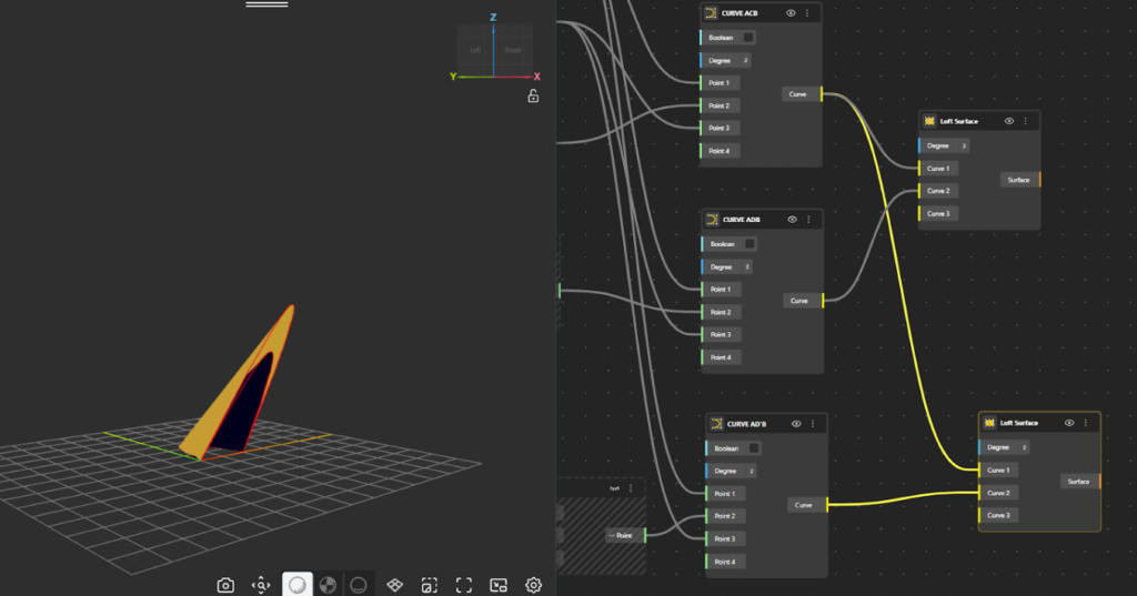
- Add NURBS Curve component to the canvas. The second curve is now defined, passing through A → D’ → B, forming a spatial (3D) curve.
- Set Point A as Point 1 of the curve.
- Set Point D’ as Point 2 of the curve.
- Set Point B as Point 3 of the curve.
- Add a Loft surface node. Connect Curves ACB and AD’B as inputs to the Loft node. The Loft component generates a surface by smoothly interpolating between the two curves along their length. (Hide the Loft node, as the surface is only used as a reference and we now want to establish a net like structure from the underlying geometry.)
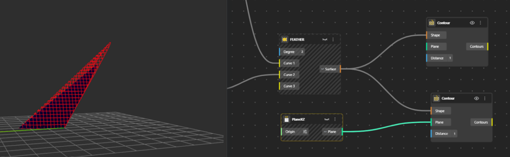
Convert the Top Structure into Feather like Structure
To create a net or feather-like structure, add a Contour component to the canvas.
- Connect the Surface (from the loft surface outport) to the Contour input.
- Define a distance value for the contour spacing.
This generates horizontal contour lines across the geometry, following its form. - For vertical contour lines, add another Contour component.
- Set the contour plane to XZ plane using PlaneXZ node for this second contour node.
- Connect the same geometry to this Contour component.
- Adjust the spacing distance until the desired net pattern appears.
- To enhance the structure, add a Pipe component.
- Connect the contour curves to the Pipe node and set the radius appropriately to give thickness.
- For a more presentable and readable structure, also connect the main curves ACB, ADB, and AD′B to the Pipe component.
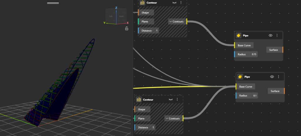
The result is a netted, feather-like spatial structure defined by intersecting contour lines. You can find the Model here.
About Ms Florina Pantilimonescu-Cioancă
Ms Florina Pantilimonescu-Cioancă is an architect, dedicated to blending creativity with data-driven approaches. She has a vast mathematical background centered around analytic and differential geometry, probability, and statistics. Today, her research aims at bridging the gap between architecture and mathematical knowledge, with a particular focus on machine learning.