A Complete Guide to CAM View in BeeGraphy

You’ve finished your parametric model. Every curve resolved, every parameter dialed in. But a model isn’t a part until a machine can cut it. That last step is what CAM View handles: it is the bridge between the geometry you designed and the physical object a CNC router or mill will produce. This guide walks the whole path, from flat profiles to a downloadable G-code file you can run.

What CAM View is . . .

In most workflows, design and manufacturing live in two different programs. You model in a CAD tool, export a neutral file, then re-import it into a separate CAM package to generate machine instructions. Every hop is a chance for something to drift: units, scale, a lost layer.

CAM View closes that gap. Because your geometry is already parametric and already in BeeGraphy, you prepare it for manufacturing in the same environment you designed it in. You assign cutting operations, pick the machine, generate the code, and verify it by simulation without leaving the platform. And because the model stays parametric, changing the design updates the manufacturing output with it.

Before you start

Before you start: setting up the workspace

Three pieces of one-time groundwork before any model can produce G-code.

1. Install the Nesting plugin. Available from the BeeGraphy Plugin Manager, it adds the nesting nodes: Rectangular Nesting for fast box-based layouts and True Shape Nesting for packing real contours.
2. Install the Machine nodes. Also from the Plugin Manager, the Manufacturing package adds the machine nodes to your editor, found under the Manufacturing group in the node menu or via search.
3. Add your machines. They’re set up as profiles in the Business Dashboard, at Workspace → Manifacturing → Machines.
   • Click the add icon, select your machine, and define its parameters: working area, spindle capacity, feed rates, Z-axis setup, and the post-processor that translates toolpaths into that machine’s own code dialect.
   • Note that machine profiles are currently created by administrators and provided to business clients, so regular users select from the predefined list rather than building profiles from scratch.
   • For the full walkthrough, see the Machines article in the help center.

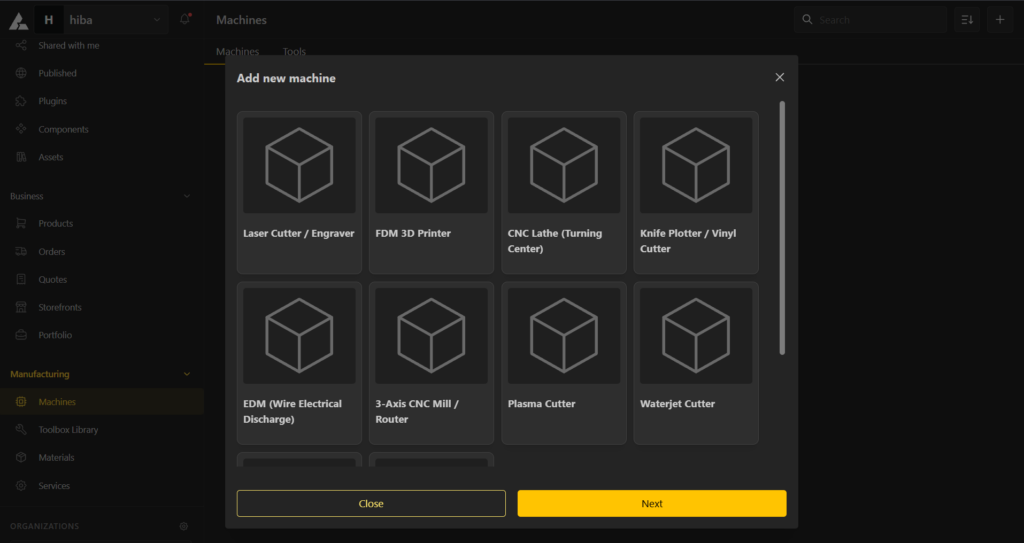
Step 1: Click on Add Icon. Select the Machine.

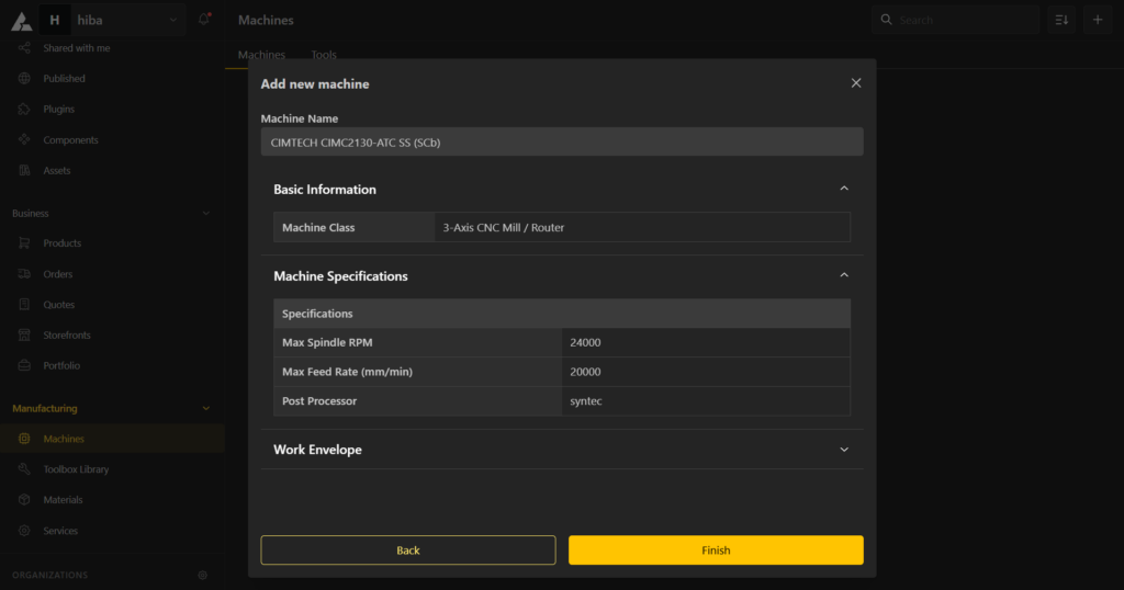
Step 2: Define your parameters and settings. Click finish when done.

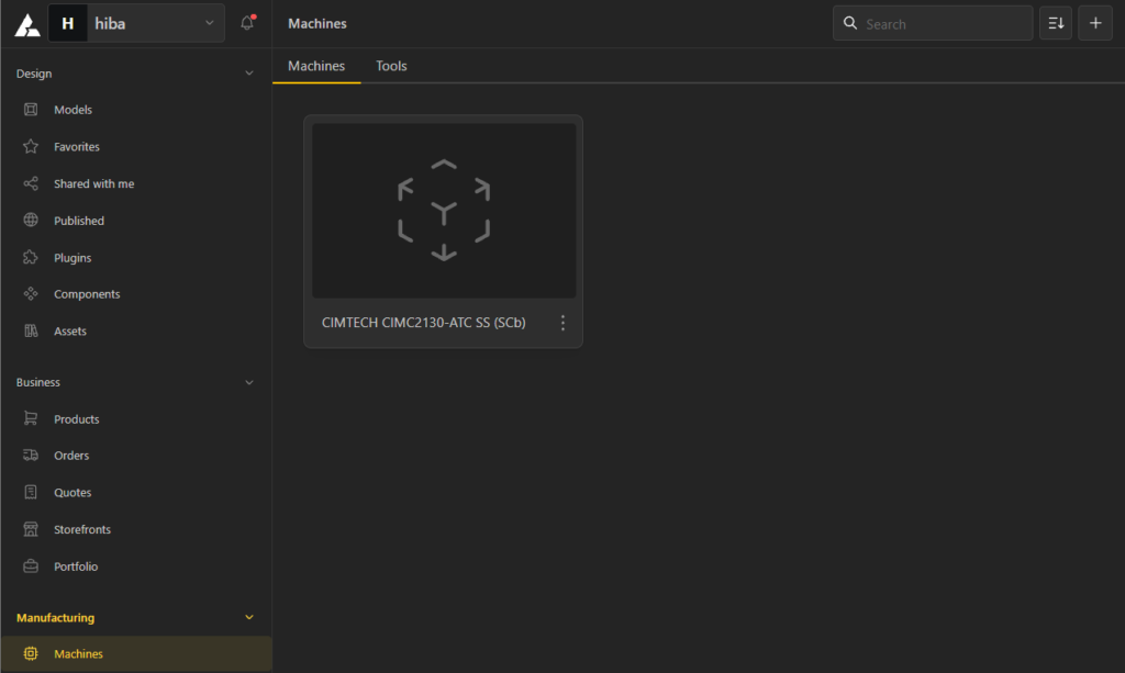
Step 3: Once added, it will show on your Dashboard under Machines.

With the plugins installed and a machine available, every model in the workspace can go from geometry to G-code.

Step 1: Get your geometry ready, 3D to 2D

Most sheet fabrication is fundamentally a 2D operation. The machine moves a tool across a flat sheet, so before anything can be cut, your 3D model has to be reduced to flat, cuttable profiles.

The first move is extracting those profiles from the model, and there’s more than one node for the job:

• Surface Edges. Pulls the boundary curves directly from a surface. The shortest path when you’re working from faces.
• Deconstruct Solid. Breaks a solid into its planes, contours, and endpoints. Since it returns everything at once, pair it with List nodes to itemize and pick out just the contours you need.
• Bounding Box with Rectangle by Center. For strictly rectangular parts, skip tracing the geometry: take the part’s bounding box and rebuild it as a clean rectangle. Simple and fast, but only when the part really is a rectangle; on anything shaped, you’d be cutting the box, not the part.

However you extract, the curves come out grouped by part, in separate lists. The nesting node needs them all in one flat list to pack them together, so pass everything through a Flatten Tree node first.

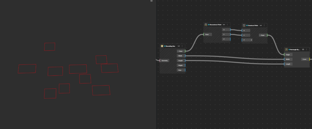
Step 2: Nesting, packing parts onto the sheet

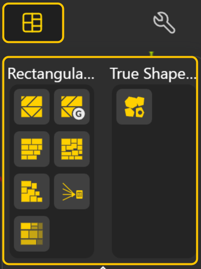
With your geometry flattened into one list, it’s ready to be packed. Nesting arranges many parts across a single stock sheet so they fit as tightly as possible. Good nesting is the difference between three sheets and two. BeeGraphy ships several nesting nodes, from quick rectangular packers to true-shape nesting for irregular contours, so pick the one that fits your parts and your machine before wiring in the settings.

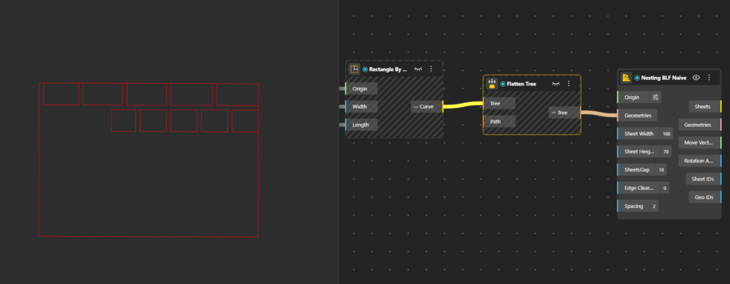
The flattened curves connect to the nesting node along with a few settings:

• Spacing. The gap between parts, the kerf or blade thickness allowance.
• Edge Clearance. The margin kept clear around the sheet edge, a trim allowance.
• Sheets Gap. The visual spacing between sheets in the output when a job overflows onto more than one; a layout convenience, not a machining setting.
• Rotation. Whether parts can be turned to fit tighter on the sheet. More rotation usually means less waste, but lock it for directional materials like wood grain or printed sheets.

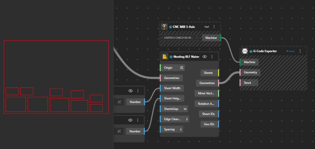
Nesting happens before the G-code step. The nested layout is what everything downstream works from.

Step 3: Apply Layer, giving the layout meaning

This is where the layout stops being a drawing and starts being something a machine will run. Two nodes do the work.

• Once your machine profile is set up in the workspace dashboard, that same machine becomes available as a node you can drop directly into your model. Add it in the editor and connect it into the G-code flow.
• The G-code node takes that machine plus your nested layout and writes the file. What comes out is a .gcode your operator can run, generated from the same graph that made the design.

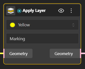
• Feeding both is the Apply Layer node, which gives them what they need to work with. It color-codes every curve by the job the machine performs there: red for cutting, blue for internal cuts, green for engraving, yellow for marking, magenta for hatching, cyan for annotations. Those layers are what operations bind to later in CAM View, which is how each operation knows which curves belong to it.

Step 4: Opening CAM View & Operations, the eight ways to cut

With the flow wired, the G-code node shows when it’s ready. Click it to open CAM View, the workspace where the prepared layout becomes an actual cutting job.

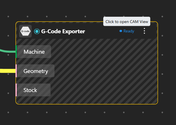
Once configured, the Ready Button will appear on the node.

The first thing to do in the new window is assign the machine. Pick from the machines defined in your workspace; this sets the working limits, feed rates, and post-processor everything downstream is built for. The same design generates different G-code depending on the machine you choose here, so it’s the first decision, not an afterthought.

With the machine set, the next job is telling it what to do with each curve. Every line on your sheet gets an operation, added as a block in the Operation Order list, and CAM View offers eight:

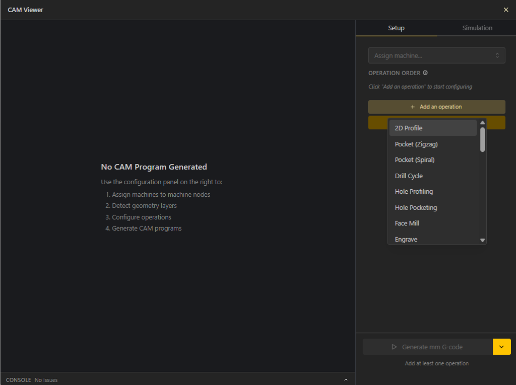
CAM View Window

• 2D Profile. The everyday “cut it out” operation: the tool follows a shape’s outline, outside the line for parts, inside for openings.
• Pocket (Zigzag). Clears all material inside a boundary with back-and-forth passes.
• Pocket (Spiral). Clears the same area with a continuous outward spiral; smoother and kinder on the tool.
• Drill Cycle. Plunges straight down at points to make holes matching the tool diameter.
• Hole Profiling. Mills a hole to size by tracing its wall, for holes larger than the tool.
• Hole Pocketing. Clears the entire circular area out when the whole disc of material must go.
• Face Mill. Skims a thin layer off the top of the stock for a flat reference surface.
• Engrave. Scores shallow lines, text, or detail without cutting through.

Order matters. Marking and engraving come first, internal cuts next, and the external perimeter cut last, so a part isn’t freed from the sheet before its other features are finished.

Step 5: Operation settings

Every operation opens its own settings dialog, organized as a sidebar of tabs. Four of them recur on almost every operation, and once you know these four you can read any operation’s dialog:

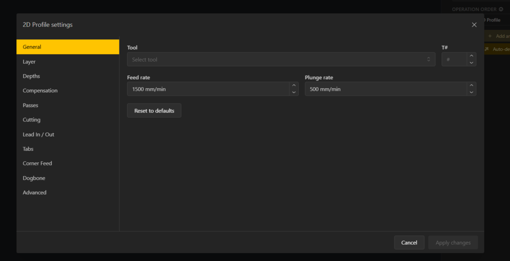
• General sets which tool the operation uses and the two rates that govern how fast it cuts. Feed rate is how fast the tool moves sideways through the material. Plunge rate is how fast it moves straight down, and it’s almost always set lower, because driving the tip downward is harder on the tool than cutting sideways. Both come pre-filled with sensible defaults and can be edited per operation.
• Layer selects which geometry the operation runs on. You can also select only part of a layer, filtering edges by corner type, angle, curvature, or length, for cases where an operation should touch only certain edges rather than the whole outline.
• Depths (called Heights on the drill and hole operations) defines the vertical stack: the safe travel heights, the top of the stock, the total cut depth, and the step down, which is how much material is removed per pass. Deeper cuts are taken in layers.
• Cutting sets the direction: Climb, Conventional, or Auto. Climb usually leaves a cleaner finish on modern machines.

Beyond these, each operation carries its own tabs for its own job. A few worth knowing on 2D Profile, since it’s the one you’ll use most:

• Compensation offsets the path by the tool’s radius so the part finishes at the right size, and lets you choose whether the software or the machine’s controller computes the offset.
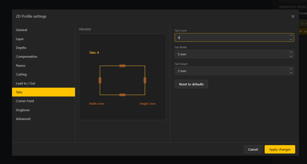
• Tabs adds small uncut bridges that hold the part in the sheet so it doesn’t break free and shift mid-job.
• Lead In/Out eases the tool into and out of the cut with an arc or tangent move instead of plunging straight in.
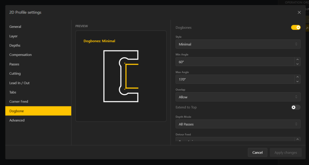
• Dogbone adds the corner relief that lets a round tool clear a sharp inside corner, so mating parts actually seat.

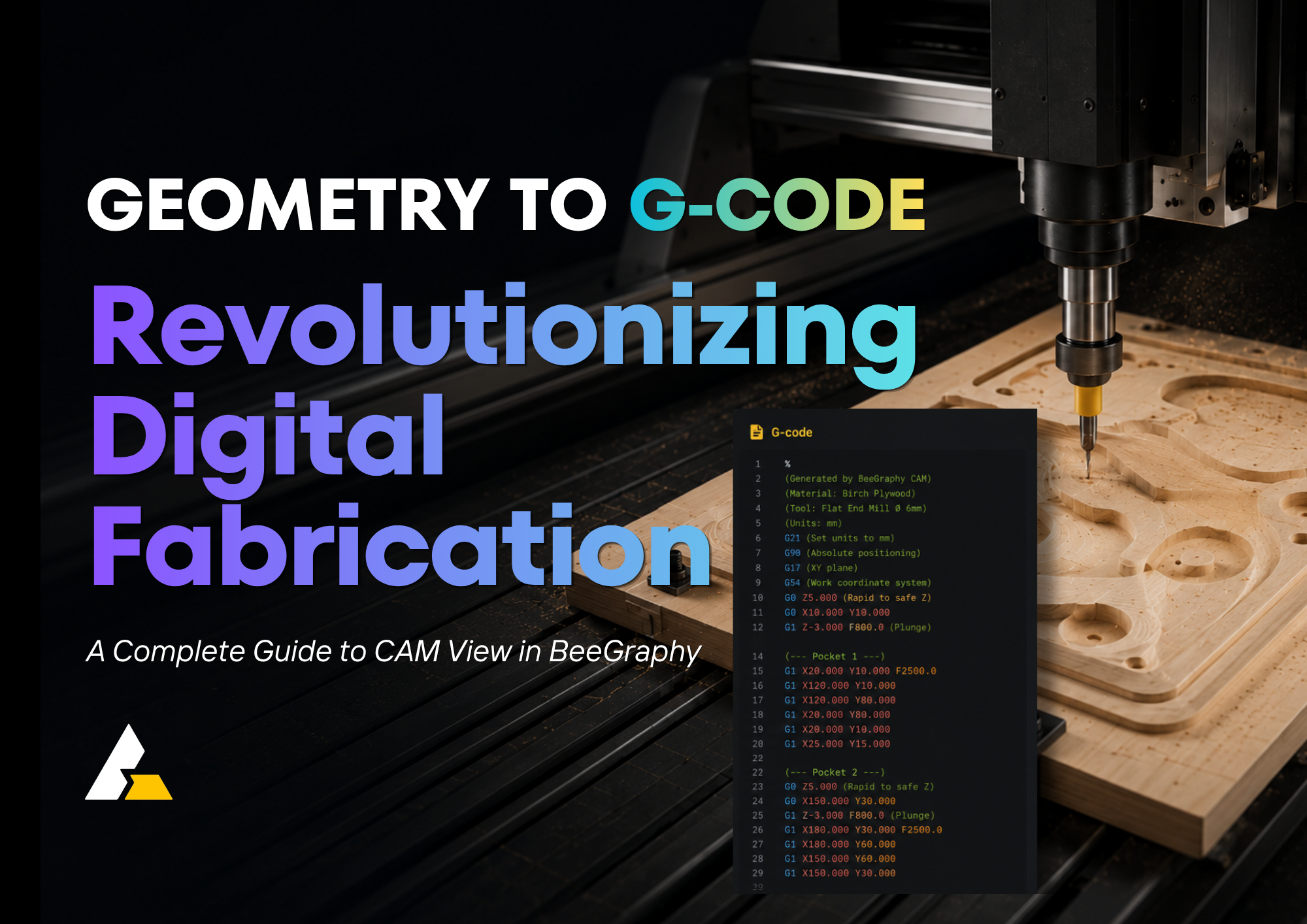
All of this exists for one reason: everything you set here is what ends up written as G-code, the plain-text instruction set your machine actually reads. Each line is either a movement, a coordinate the tool travels to, or a command that changes the machine’s state, like starting the spindle or changing tools. Feed rate, plunge rate, cut depth, tool number: every setting above becomes a value in that code. So the settings aren’t abstract, they’re the exact numbers the machine will move by.

Step 6:Generate the G-Code, and watch Simulation in real time

Once your operations and their settings are in place, click Generate. This builds the simulation and, if anything’s missing, an operation without a layer, a setting left incomplete, an error shows here first, before it ever reaches the machine. With generation successful, the simulation plays back the toolpath, so you can watch the entire job before a single cut happens on real material.

What you’re actually looking at:

• The geometry. Your part, sitting on the stock, exactly as it was nested and laid out on the sheet.
• The toolpath. The route the tool follows for every operation, in order, colored by operation so a profile cut, a pocket, and an engrave are easy to tell apart at a glance. Watching it move shows you not just where the tool goes, but when: which curve gets cut first, which gets cut last.
• Rapids vs. cuts. The simulation distinguishes fast repositioning moves, where the tool lifts clear and travels without touching the material, from the actual cutting moves. Seeing both helps you catch wasted travel or a tool passing somewhere it shouldn’t.

Playing it through is the cheapest place to catch a problem: a cut in the wrong order, a missed profile, a tool diving too deep. If Generate throws an error instead, that’s the workspace telling you something upstream needs fixing, material, machine, or a layer assignment, before it will even build the preview.

All of this exists for one reason: everything you set here is what ends up written as G-code, the plain-text instruction set your machine actually reads. Each line is either a movement, a coordinate the tool travels to, or a command that changes the machine’s state, like starting the spindle or changing tools. Feed rate, plunge rate, cut depth, tool number: every setting above becomes a value in that code. So the settings aren’t abstract, they’re the exact numbers the machine will move by.

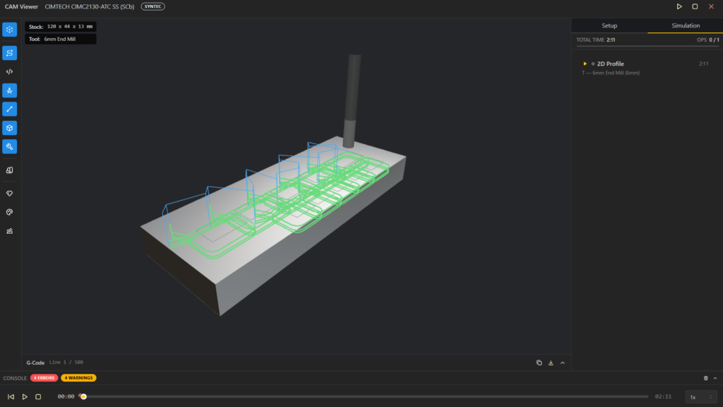
The simulation view gives you a set of inspection controls:

• View toggles let you switch to a flat 2D top-down view, hide the toolpath, the stock, the tool, or the original geometry, and hide rapids (the fast non-cutting repositioning moves) to declutter the display.
• Operation colors shade each path by the operation it belongs to, so profiles, pockets, and drills are easy to tell apart at a glance.
• Playback controls let you play, pause, stop, and change speed, so you can scrub through a long job quickly or slow down to watch a tricky section.

Step 7: Generate and download

When the simulation looks right, Download the G-Code. The post-processor translates the toolpath into the exact syntax your machine’s controller understands, and the result is a G-code file you can copy to the clipboard or download directly from the simulation view. Load it on the machine, and the part you modeled becomes the part you hold.

One last thing

CAM View is under active development; a few features are still evolving, and we’re improving them with every release. A full video tutorial is on the way too. In the meantime, if you have questions or run into anything unclear, reach out to us; we’re happy to help you get from geometry to G-code.