AI Parametric Design: 6 Easy Steps to Reaction Diffusion

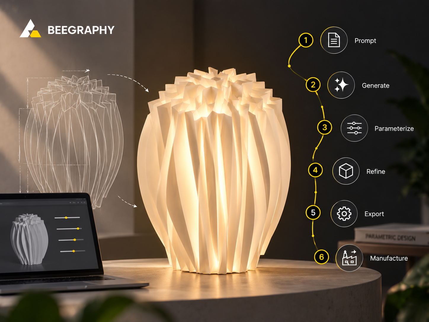
AI parametric design turned reaction diffusion into curves you can build with. Here is the BeeGraphy node, a lamp made from it, and the free prompt.

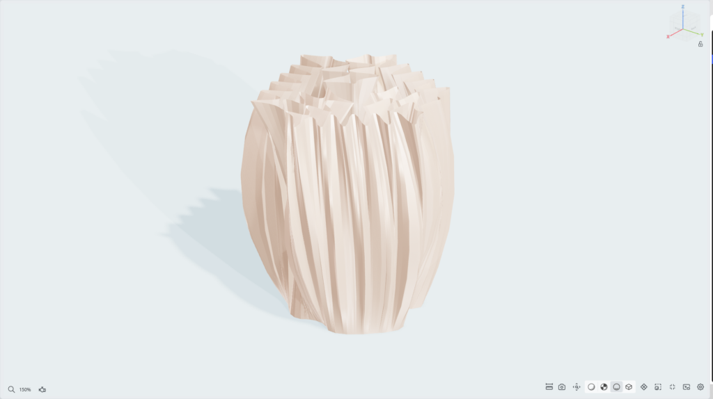
A product, not a pattern study. The profile came straight out of the reaction diffusion node.

Why we wanted reaction diffusion for products

Reaction diffusion is everywhere in computational design imagery and almost nowhere in computational design products.

The reason is boring and practical. Most reaction diffusion implementations output a pixel field or a mesh soup. Beautiful on screen, useless downstream. You cannot loft it, you cannot offset it for wall thickness, you cannot hand it to a CNC.

What a product workflow needs from reaction diffusion is a clean closed curve. One that does not cross itself, sits on a plane, and lofts without argument.

No node does that. So we built one, and we let AI parametric design do the writing.

What reaction diffusion actually is

Two chemicals sit in the same space. One activates, one inhibits. Both diffuse, at different speeds.

Where the inhibitor spreads much faster than the activator, the system settles into Turing patterns: peaks at a characteristic spacing. Pufferfish skin, coral, fingerprints.

We used the Gierer-Meinhardt form of the reaction diffusion equations, running along the arc length of a closed curve rather than across a surface.

a_t = Da·a'' + ρ·a² / (h·(1 + κ·a²)) − μa·a
h_t = Dh·h'' + ρ·a²                   − μh·h

Each sample point then moves along its own normal by the local activator concentration. High activator, the curve bulges outward. Low, it pulls in. The lobes land at the spacing the chemistry dictates, not at a spacing you drew.

Letting AI parametric design write the node

BeeGraphy’s TypeScript node takes a function, exposes ports, and behaves like any other component on the canvas. That is where the solver lives.

We described what we wanted to Claude in plain English. Not specifications. The kind of thing you say to a colleague.

“do not make the curve collide with itself”

“the curve should move till they do not collide”

“it is working perfect but is making the script slower, can we make it faster?”

That last one produced a counting-sort spatial grid and a fast-path early exit, making the node nine times faster. We never asked for either by name. We said it was slow. That is what AI parametric design feels like in practice.

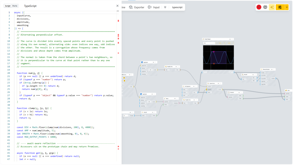
The instruction on the left. The solver on the right.

The bug that nearly shipped

The node ran. It produced beautiful organic lobes. We iterated on it for hours.

Then we asked the model to measure one diffusion constant instead of estimating it. While printing diagnostics it also printed the pattern contrast, which came back as zero to three decimal places.

So it ran a linear stability analysis. A two-chemical system only forms Turing patterns if the inhibitor diffuses far enough faster than the activator. There is a hard threshold, and for our reaction rates it sat around 80.

required  Dh/Da  >  ~80
ours      Dh/Da  =   40

Our simulation had never run. The activator array was flat to six decimal places. Normalizing that flat array stretched float rounding noise to full amplitude, and smoothing turned the noise into convincing organic waves.

We had been admiring our own rounding errors, while every visual check passed.

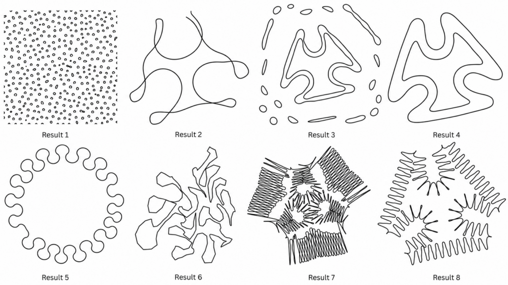
AI Parametric Design: From Reaction–Diffusion to Form.

Raising the inhibitor diffusion to 0.8 against an activator at 0.004 put the ratio at 200. Pattern amplitude went from about one part in a million to 2.4, and the wavelength held steady at 11 cells across every grid size we tested.

This is the central lesson of AI parametric design. A good render proves nothing. Three habits came out of it, and all three are in the prompt:

1. Ask for derivations. If the script encodes physics you did not derive, make the model derive the conditions and check your numbers against them.
2. Never let it grade its own homework. We ran a brute-force checker written separately from the solver. If they disagreed, the solver was wrong.
3. Demand a fuzz harness. We ran 2,400 randomized cases. Zero self-intersections.

What the BeeGraphy node gives you: curves you can build with

The output is a single closed curve, guaranteed non-self-intersecting, planar, and emitted as a one-edge B-spline so it lofts against anything.

Six inputs control it: inputCurve, amplitude, patternScale, iterations, direction and seed. Pattern scale sets lobe size. Iterations deepen the growth. Seed makes the whole thing reproducible, so a slider change upstream does not reshuffle your pattern.

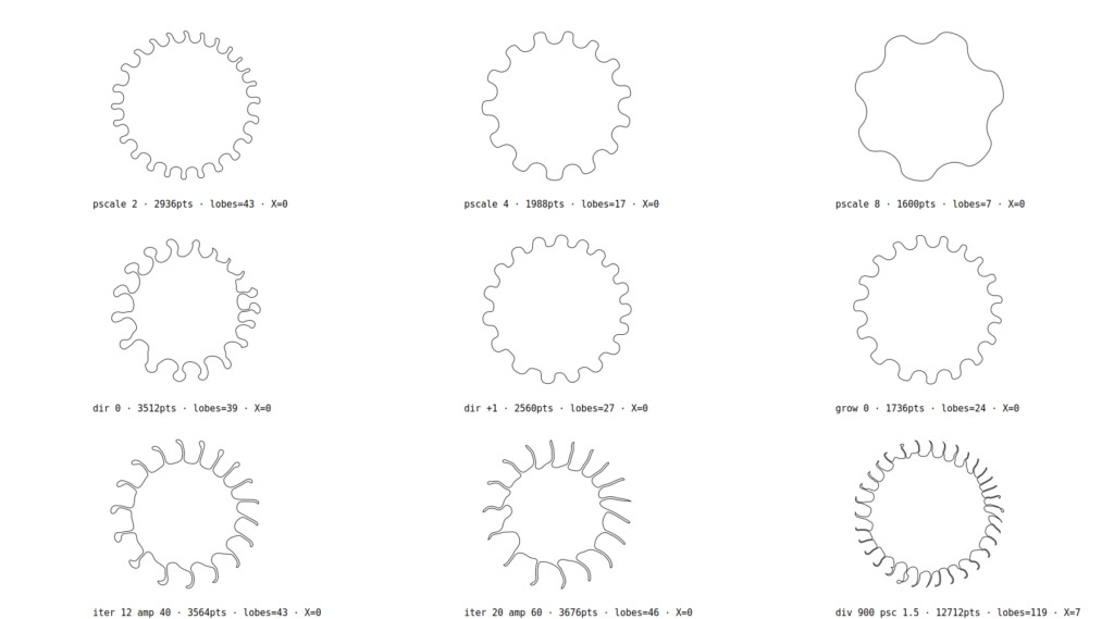
One node, one input curve. Pattern scale from 1 to 12.

Because it is a real curve rather than a field, everything downstream just works. Offset it for wall thickness. Loft it. Extrude it. Send it to CAM.

Case study: turning reaction diffusion curves into a lamp

To show the pipeline end to end, we made a lamp shade.

Two reaction diffusion profiles, generated from the same base curve at different settings. One for the bottom, one for the top, moved up in Z. Tween Curve fills in every section between them, so the silhouette is interpolated rather than modelled. A Graph Mapper on a sine curve drives a Scale node centered on each section’s own centroid, which produces the flare. Then Loft Surface.

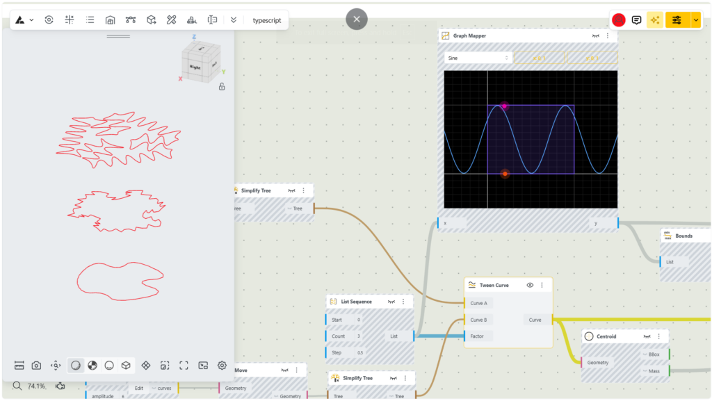
Two reaction diffusion nodes, a tween, a sine profile, a loft.

The principle worth taking from this: script the part that needs memory, node the rest. The solver produces one good curve. The graph does the interpolating, remapping and lofting, because that is what graphs are best at.

Build it in 6 easy steps

1. Open a new file in the BeeGraphy editor. Add a Star, a Discontinuity, and a NURBS Curve set to Periodic and Clamped at degree 3.
2. Add a TypeScript node. Create input ports named inputCurve, amplitude, patternScale, iterations, direction, seed, and one output port named curves.
3. Paste our prompt into Claude and let it run. Ask to see the fuzz test output before you accept anything.
4. Paste the result into the TS Code field. Two gotchas: async must be the first character, and no semicolon after the closing brace.
5. Wire the curve in. Start at amplitude 20, patternScale 3, iterations 5.
6. Duplicate the node with different settings, Move one up in Z, Tween Curve between them, then Loft Surface.

You do not have to build it from scratch to try it. Open our finished lamp file in BeeGraphy
Reaction Diffusion Lamp

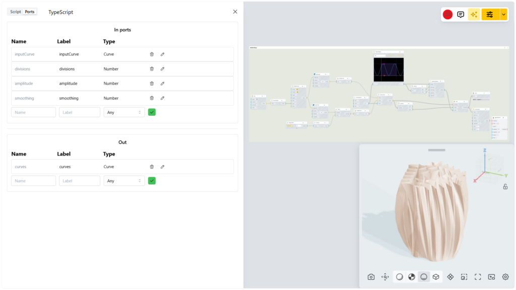
Six ports. Names must match the prompt exactly.

Get the free AI parametric design prompt

There is no magic one-shot prompt. Ours took ten rounds and three bugs the model found in its own work. But those rounds compress into a spec you can reuse.

Write one TypeScript script node for BeeGraphy (browser parametric CAD, OCCT kernel). 

## Environment — tested, do not deviate - One bare async arrow fn: async ({ portA, portB }) => { ... }. async must be the FIRST character — no leading comment or blank line (the editor prepends return; ASI breaks it). No trailing semicolon. - No type aliases, no param type annotations ("type is not defined"). - No spread, ??, optional chaining, or .map() with complex arrows. Plain for loops. Nested function declarations, typed arrays, dynamic string keys are fine. - Port names are JS variables: valid identifiers, case-sensitive. Unconnected = null. - Return { type: Type.Curve, value, meta }; keys must match out-port names exactly. Points: new Vector([x, y, z]). - Curve methods are on the PROTOTYPE chain (getOwnPropertyNames won't find them) and accessors may return Promises — await every read and every builder call. - Curve: divideByCount, divideByLength, pointOnCurve, evaluateCurve, curveToPolyline, controlPoints, curveLength, getDividedSegments, startPoint, endPoint, isClosed. Builders: CurveBuilder.polyline, CurveBuilder.bSplineCurve — probe for anything else. 

## Task — corrugate a closed planar curve In: inputCurve (Curve), divisions (Number, 200), amplitude (Number, 5), smoothing (Number, 0), outputForm (Number, 1). Out: curves (Curve). Divide evenly; push each point along its own normal, alternating side by index parity. The normal comes from the chord between a point's two NEIGHBOURS, not from either adjacent segment. 

## Non-self-intersection — never, not "usually" Implement as growth, not offset-then-repair. Every point starts flat at scale 0 and advances to full amplitude in 20 equal increments; after each, rebuild the entire curve and scan for collisions. Any point in a collision rolls back one increment and freezes permanently. Each rib travels as far as it can and stops at contact. 1. Freeze ONLY points actually in contact. Freezing neighbours cascades along the curve and stalls everything in the first few steps. Widen to neighbours only when every contacting point is already frozen and there is nothing left to roll back. 2. Smoothing goes INSIDE the rebuild, or you verify one curve and ship another — Chaikin corner-cutting can land a cut across a segment the sharp version cleared. 3. Clamp offset toward the concave side to 0.8× local radius of curvature (circumradius of three consecutive points). No clamp when moving away from the centre of curvature. 4. Reject an input that already self-intersects — say so rather than emit something broken. 

## Verification — show me the output, don't tell me it works - Brute-force O(n^2) segment intersection checker OUTSIDE the node. Different algorithm, no shared code. If the two disagree, the solver is wrong. - Fuzz harness: random closed curves from random radial harmonics, deliberately uneven sampling, random divisions/amplitude/smoothing. ≥600 cases per seed, several seeds. Report every failing case. - Final de-looping backstop: cut at any surviving intersection, discard the smaller loop. Capped iteration is not a proof; this is. 

## Output form outputForm 1 → single-edge B-spline. (A polyline at 200 divisions with smoothing is thousands of edges; BRepFill_CompatibleWires can't reconcile that against a four-edge section and SurfaceBuilder.loft fails.) The guarantee is proved on the polyline, and the spline is a different curve that can bulge outside it — run a dense Catmull-Rom approximation of it through the same collision scan, and fall back to the polyline if it fails. 

## Performance - No O(n^2) scan per step: flat counting-sort grid over reused typed arrays. Not a plain object keyed "gx_gy" — that's a string concat, hash lookup and allocation per segment per cell. - Grid cell size bounded to ≥100 cells across the bbox, or large amplitude buckets everything into one cell. - Try full amplitude ONCE before the growth loop; most curves have room everywhere. - Skip segments unmoved since the last clean scan. This breaks any adjacency test written b <= a + 1, which assumes the scan visits every segment in order — measure separation properly in both directions or you silently stop testing real pairs. - Preallocate every buffer; the rebuild runs ~35× per solve. 

## Diagnostics meta on the output, at minimum: selfIntersections (must be 0), averageReach and maxReach as fractions of requested amplitude, pointsOut, edgeCount, outputForm, amplitudeClamped, loopsRemoved, buildMethod. A bad result must be diagnosable from the numbers alone. 

## Port robustness The curve may arrive bare, array-wrapped, in a { value: ... } envelope, nested several levels, or as a Promise. Walk all of those recursively. Identify it by whether it exposes curve methods, not by guessing the wrapper shape. Accept a raw point list as fallback. On failure the error must say what actually arrived.

Read its shape, not its words. A third is environment constraints. Another third is verification. The algorithm itself is eight lines, and there is almost no description of what the result should look like.

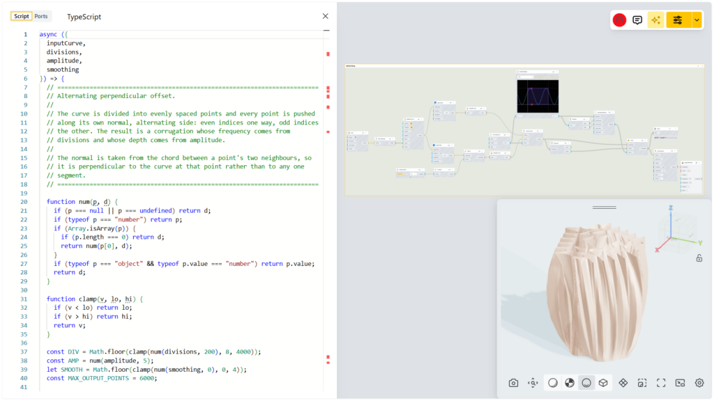
AI parametric design script node and node graph building a ribbed lamp shade in BeeGraphy

Good AI parametric design prompts describe constraints, failure modes and proof. Swap the algorithm section for your own idea and the rest still works.

Now go break it

Run it on a non-circular base. Chain two nodes at different pattern scales. Push the amplitude until the solver fights back, then screenshot it.

Post what you make and tag us. Post what you break, too.

The whole build took an afternoon. Barely any of it was writing code. Almost all of it was working out what the code had to prove.

AI parametric design FAQ

Do I need to know how to code for AI parametric design?
Not to write it. You need to read it and know what to ask for. Every decision that mattered here was design and verification, not syntax.

Why did the reaction diffusion code fail when the output looked correct?
The diffusion ratio was below the Turing threshold, so no pattern could form. The node was amplifying float rounding noise, and it looked convincing.

Can the output be manufactured?
Yes. That was the point. It is a clean closed planar curve with no self-intersections, so it offsets, lofts and exports like any other curve in BeeGraphy.

How do I stop AI parametric design geometry from self-intersecting?
Do not ask the model to avoid it. Ask it to prove the output is clean, with a checker written separately from the solver, run across hundreds of randomized inputs.

Is the output reproducible?
Yes. The seed input makes the solver deterministic, so changing an unrelated slider will not reshuffle your pattern.

How fast is the node?
Typically well under a second. The worst case we could construct runs in a few hundred milliseconds.

Does this work outside BeeGraphy?
The method transfers anywhere with a scripting node. Only the curve sampling and wire building use the OpenCASCADE kernel bindings that BeeGraphy is built on.

Want to get good at the part AI cannot do for you? CD101 teaches the computational design thinking behind every judgment call in this article.

Computational Design 101 — Learn the fundamentals and build a parametric mindset with BeeGraphy.